
Before Word2Vec, representing words for ML was painful. One-hot encoding treated every word as equally different. TF-IDF captured some statistics but no meaning. Then in 2013, Mikolov and team at Google published Word2Vec, and suddenly we could do things like:
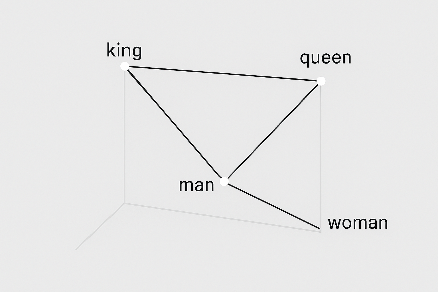
king - man + woman ≈ queen
Wait, what? Word arithmetic that actually works? Let’s see how.
The brilliant insight
Words that appear in similar contexts have similar meanings.
Think about it: “dog” and “cat” both appear near words like “pet”, “cute”, “fur”, “feed”. The word “laptop” appears near totally different words. So if we train a model to predict context, “dog” and “cat” vectors will naturally end up close together.
The embeddings aren’t the goal - they’re a “side effect” of training a simple prediction task. And that side effect turned out to be incredibly useful.
Interactive demo: Word2Vec Animation - see how word vectors organize themselves during training.
Two training flavors
Skip-gram: Given a center word, predict the surrounding context words
"The cat sat on the mat"
Center word: "sat"
Predict: "The", "cat", "on", "the"
CBOW (Continuous Bag of Words): Given context words, predict the center
Context: "The", "cat", "on", "the"
Predict: "sat"
Which is better? Skip-gram works better for smaller datasets and rare words. CBOW is faster and handles frequent words well. In practice, Skip-gram is more popular.
The architecture (surprisingly simple)
It’s basically just one hidden layer:
- Input: one-hot encoded word (vocabulary size V)
- Hidden: embedding dimension (typically 100-300)
- Output: vocabulary size V, with softmax
Input (V) → Hidden (D) → Output (V)
The hidden layer weights ARE your word embeddings. That’s it!
Negative sampling
Don’t compute full softmax. Instead:
- Real context pairs: positive examples
- Random word pairs: negative examples
Only update weights for these few words per example.
# pseudo-code
for center, context in training_data:
    loss = -log(sigmoid(dot(center_vec, context_vec)))
    # add k negative samples
    for neg_word in sample_negatives(k):
        loss += -log(sigmoid(-dot(center_vec, neg_vec)))
Much faster. Quality nearly as good.
The famous analogies
“king - man + woman = queen”
This actually works (roughly). Vectors capture semantic relationships.
# assuming we have word vectors
result = model['king'] - model['man'] + model['woman']
most_similar = find_nearest(result)  # returns 'queen'
Practical considerations
Window size
Smaller (2-5): captures syntactic similarity Larger (5-10): captures topic/semantic similarity
Embedding dimension
More dimensions = more capacity but slower and needs more data Common: 100-300 for most applications
Minimum count
Words appearing < N times get filtered. Rare words don’t have enough context to learn good vectors.
Training your own
from gensim.models import Word2Vec

sentences = [["the", "cat", "sat"], ["the", "dog", "ran"]]

model = Word2Vec(
    sentences,
    vector_size=100,
    window=5,
    min_count=1,
    sg=1  # skip-gram
)

# get vector
cat_vec = model.wv['cat']

# similar words
model.wv.most_similar('cat')
Word2Vec intuition unlocked? Consider starring ML Animations and spreading the word on social media!