Why do we use cross-entropy for classification? And what does it actually measure? Let’s break it down - understanding this will help you debug models and choose the right loss functions.
The big idea
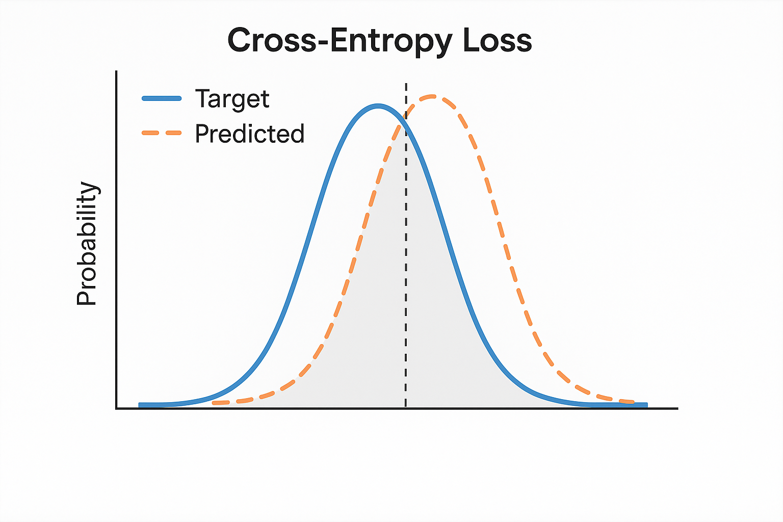
Cross-entropy measures how “surprised” your model is when it sees the true answer. If the model confidently predicted the right class, low surprise (low loss). If the model was confident about the wrong class, huge surprise (high loss).
For true distribution P and predicted distribution Q:
$$H(P, Q) = -\sum_x P(x) \log Q(x)$$
In classification, P is one-hot (true label), Q is your softmax output.
Interactive demo: Cross-Entropy Animation - watch how loss changes as predictions shift.
A concrete example
Say we have 4 classes and the true label is class 2.
True label (one-hot): [0, 0, 1, 0]
Model prediction: [0.1, 0.2, 0.6, 0.1]
$$\text{Loss} = -\sum_i y_i \log(\hat{y}_i) = -\log(0.6) = 0.51$$
Notice something? Only the true class matters! Everything else multiplies by 0.
So cross-entropy is really just: $-\log(\text{predicted probability of true class})$
Why this makes sense
Think about what the loss does:
| Situation | Math | Loss |
|---|---|---|
| Confident and correct | -log(0.99) | 0.01 (good) |
| Unsure but correct | -log(0.5) | 0.69 |
| Slightly wrong | -log(0.3) | 1.2 |
| Confident and wrong | -log(0.01) | 4.6 (bad) |
The key insight: cross-entropy heavily punishes confident wrong predictions. This is exactly what we want - it forces the model to be careful about what it’s confident about.
Binary cross-entropy
For binary classification with sigmoid output:
$$\text{BCE} = -y\log(\hat{y}) - (1-y)\log(1-\hat{y})$$
The first term handles “should be 1” cases, the second handles “should be 0” cases.
import torch.nn.functional as F

# Binary
loss = F.binary_cross_entropy(predictions, targets)

# Or with logits (more stable - explained below)
loss = F.binary_cross_entropy_with_logits(logits, targets)
Multi-class cross-entropy
$$\text{CE} = -\sum_{c=1}^{C} y_c \log(\hat{y}_c)$$
Important PyTorch note: CrossEntropyLoss expects raw logits, NOT softmax outputs. It applies softmax internally:
loss_fn = nn.CrossEntropyLoss()

# logits: (batch, num_classes) - raw network output
# targets: (batch,) with class indices (not one-hot!)
loss = loss_fn(logits, targets)
Why we use logits (numerical stability)
Computing softmax then log separately is dangerous:
# DON'T DO THIS
probs = F.softmax(logits, dim=-1)  # might underflow to 0
loss = -torch.log(probs[target])   # log(0) = -inf, crashes!
The combined log-softmax is stable: $$\log\text{softmax}(z_i) = z_i - \log\sum_j e^{z_j}$$
# DO THIS
loss = F.cross_entropy(logits, target)  # handles everything safely
Label smoothing
Instead of hard one-hot [0, 0, 1, 0], use soft [0.025, 0.025, 0.925, 0.025].
Prevents overconfidence. Regularization effect.
loss_fn = nn.CrossEntropyLoss(label_smoothing=0.1)
Class imbalance
Some classes rare? Weight the loss:
# Classes weighted inversely to frequency
weights = torch.tensor([0.1, 0.3, 1.0, 0.5])
loss_fn = nn.CrossEntropyLoss(weight=weights)
Focal loss
For extreme imbalance. Down-weight easy examples:
$$\text{FL} = -(1-\hat{y})^\gamma \log(\hat{y})$$
Easy examples (high ŷ) contribute less.
# Not in PyTorch by default, but easy to implement
def focal_loss(logits, targets, gamma=2.0):
    ce = F.cross_entropy(logits, targets, reduction='none')
    pt = torch.exp(-ce)
    return ((1 - pt) ** gamma * ce).mean()
Cross-entropy loss demystified? Give ML Animations a star and help others understand these concepts by sharing!